Metric Space Methods
Introduction
In mathematics, a metric space is a set where a distance (called a metric) is defined between elements of the set. Metric space methods have been employed for decades in various applications, for example in internet search engines, image classification, or protein classification. For general background information on metric spaces, please refer to this Wikipedia page.
In petroleum reservoir modeling, metric space methods are not widely known, and few applications of metric space methods have been presented. Most all the work using Metric Spaces has come from the Stanford Center For Reservoir Forecasting under guidance of Prof. J. Caers. The slow adoption is likely due to the fact that the vast majority of reservoir modeling studies are performed using a single (static) reservoir model, which is calibrated to historical data and then used for analysis and decision making. In such cases, there is no possibility to quantify the uncertainty in the forecast that comes comes from the uncertainty associated with the input: geology, initilization, PVT, relative permeabilities, etc.
Overview
Metric space methods are best employed to analyze and interpret a group (ensemble) of reservoir models and are attractive methods for uncertainty studies or sensitivity analysis when a (large) ensemble of reservoir models is used.
A metric space (MS) in reservoir modeling is defined by a dissimilarity distance which measures the dissimilarity between pairs of reservoir models, shown schematically in the figure below (left). The distance measure applied over all model pairs forms a distance matrix shown in the figure below (center). The distance matrix defines the metric space. The metric space can be visualized using multi-dimensional scaling (MDS), whose output is shown in the figure below (right). MDS takes the distance matrix, and translates the models into points in a Euclidean space that can be visualized. The location of the points (models) in Euclidean space are optimized to best approximate the distances in the distance matrix. The MDS plot is a visual and diagnostic tool. MDS is a dimensionality reduction technique, similar to PCA.
|
|
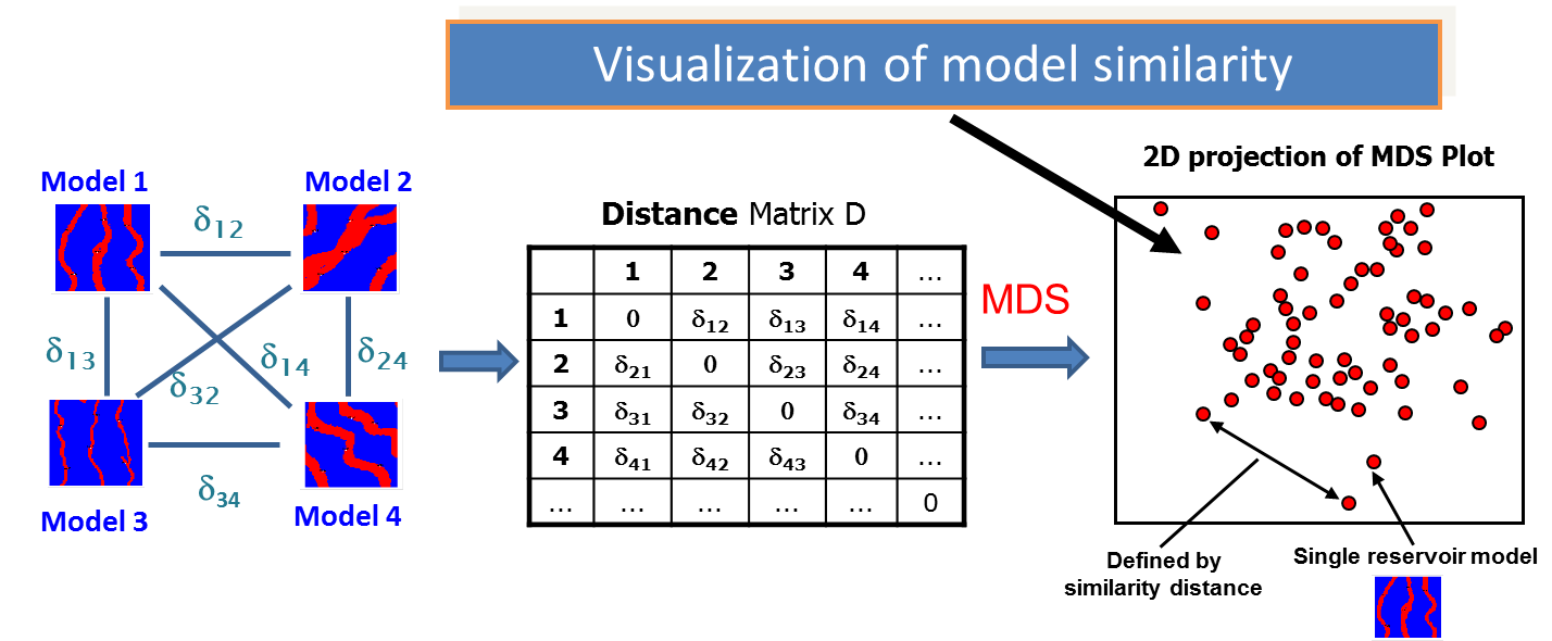
As is illustrated above, the distribution of the models in Euclidean space provides a visualization of the model similarity - models close to each other in MDS space are similar in terms of the distance measure. Those models far from each other are dissimilar in terms of the distance measure.
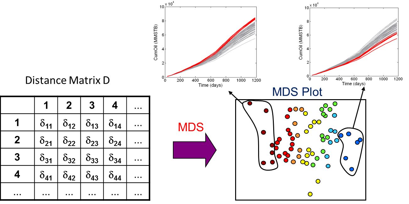
Another important step for sensitivity analysis and screening of reservoir models is clustering of the reservoir models. Clustering of the models allows for a classification of models into discrete groups. This is useful for sensitivity analysis (comparing model properties within each cluster and between clusters), and screening (selection of models based upon cluster).
An illustration is shown in the figure below. The models in the MDS plot are colored by cluster. The clustering has grouped together models with similar cumulative oil production, as seen in the figures above the MDS plot. Given this information, one can examine the model properties in each cluster and understand which properties have a significant impact on the cumulative oil.
|
|
What is a Distance?
The creation of a metric space requires the definition of a dissimilarity distance, which measures the dissimilarity between two different models. The distance measure has two main requirements. First, since the distance must be calculated between each model pair, it should be rapid to calculate for large ensembles of models. Second, the distance measure must be designed for the purpose of the study to be undertaken. No single distance measure is applicable to all situations. Finally, the distance measure must be easy to understand, in order to understand the results of the study.
What distance measure should one use for a particular study? Often the solution is clear. For sensitivity analysis and screening for history matching purposes, most likely a distance using flow simulation is appropriate. For a study of uncertainty, static property-based distances have been used. Or, one can use a combination of distances, first a static property-based distance, then a flow-based distance. Some examples of distances follow.
Static-Based Distance Measures
One distance measure which has been commonly used in the past, yet not recognized as a distance, is the total pore volume, or OOIP of the reservoir model. Total pore volume is often used in ranking of reservoir models and model selection for uncertainty quantification or history matching. Static property-based distances such as this are attractive because they are fast to computer, since there is no flow simulation required. However, static-based distance measures can go beyond global properties such as total pore volume or OOIP.
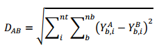 One example of a grid-based distance measure is shown on the right. Here, the variable Y is the grid property, nb is the number of grid blocks, and nt is the number of time steps (if the grid property is a dynamic property such as water saturation). One example of a grid-based distance measure is shown on the right. Here, the variable Y is the grid property, nb is the number of grid blocks, and nt is the number of time steps (if the grid property is a dynamic property such as water saturation). |
A grid-based distance may be attractive if there are many models, flow simulation per model is expensive, and the modeler wishes to reduce the large set of models by selecting diverse models based upon some static measure (like pore volume or oil volume per block). However, if the goal of the sensitivity study or screening is to distinguish models based upon flow response, there is a question about whether a static-based distance is appropriate. The answer depends on the study in question and the specifics of the reservoir model and displacement.
Flow-Based Distance Measures
Because most of our studies involve flow simulation, a flow-based distance measure will most likely be an appropriate choice. Flow-based distances can account for dynamic properties such as relative permeability curves, phase properties (viscosity, Bo), and phase contacts, in addition to model heterogeneity and barriers to flow. However, there may be many models in the ensemble, and flow simulation on each model may be very CPU demanding depending on the reservoir model. For this reason, streamline simulation has been used as an effective flow-based distance measure, since it is known to be less CPU-intensive compared to standard flow simulation, and acts as a good proxy for flow simulation using standard simulation techniques (see for example, Scheidt & Caers 2009 SPE-118740-PA).
One extremely rapid flow-based distance measure which employs streamlines is the connectivity-based distance:
|
where Y is a flow measure between an injector/producer pair (such as the total rate), nc are the number of source/sink connections at a time step, and nt are the number of time steps in the simulation. |

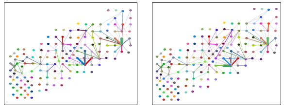 |
In essensce, the equation above calculates the difference between two FPmaps at a given time step (examples of FPmaps are shown to the right). This distance may be useful when examining the effect of different fault interpretations or depositional scenarios on the connectivity between producing wells and supporting injectors/aquifers. One major advantage is that only a single time step (snap-shot) is required to obtain a FPmap, so a full flow simulation is not required.
For studies involving history matching or uncertainty quantification of one or more flow responses, one may want to use a distance measure which employs flow simulation. Note again however that for large ensembles, these types of distance measures may be CPU intensive, therefore fast flow simulation techniques like streamline simulation may be of interest. Recall that one of the important requirements of a distance measure is that it must have relevance to the study to be performed. For example, a static grid block based distance measure may poorly distinguish the difference in water breakthrough times for different reservoir models. However, a streamline-based distance measure may be well correlated to the difference in water breakthrough times, as in Scheidt & Caers 2009 SPE-118740-PA.
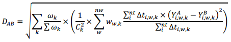
A flow-based distance measure is shown below. This expression represents a time-step-weighted, root mean-squared value of the differences of a well variable Y over nt time steps. For sensitivity analysis or history matching of flow response, this would be an appropriate distance measure.
|
|
Flow-Based Distances and History Matching
The expression above is very similar to the well-known expression for the objective function used in optimization methods such as history matching. The main difference is that an objective function is a distance measure between a model and historical (observed) data, whereas the above expression measures the distance between two models.
When a flow-based distance is being used, or indeed, whenever any observed property of the reservoir is employed in a distance measure, we can add an additional row and column in the distance matrix containing the distance between each reservoir model response and the observed (historical) data.
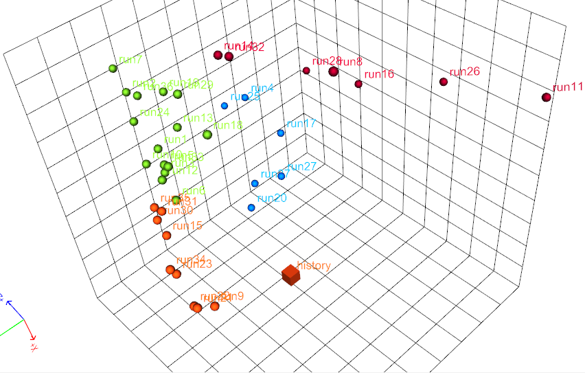
The result is that, although there is no reservoir model associated with the historical data, it can be added to the metric space. One clear benefit of this is that when visualizing the metric space using MDS, we can plot the historical data with the ensemble of reservoir models which were created. The figure on the right shows an example, where 37 reservoir models were created, and the dissimilarity distance measure is the well-level oil production rates. The simulated rates are compared to the historical rates , and the history is shown as a cube in the middle of the plot. |
Contact in USA
Corporate Headquarters 
StreamSim Technologies, Inc.
865 25th Avenue
San Francisco, CA 94121
U.S.A.
Tel: (415) 386-0165
Contact in Canada
Canada Office 
StreamSim Technologies, Inc.
Suite 102A - 625 14th Street N.W.
Calgary, Alberta T2N 2A1
Canada
Tel: (403) 270-3945