Streamline-Based History Matching

Streamlines connect reservoir regions to well production mismatches over time. Streamsim Technologies spent over 10 years in R&D, collaborating with Stanford University and production companies, to develop a novel workflow for individual well-level history matching. This approach modifies static gridblock properties between wells, assuming that well-level mismatches can be corrected by adjusting geological properties between wells.
The History Matching Workflow
Field-Level History Match
The starting point is to run a flow simulation over the complete history, ensuring an acceptable field-level history match of oil, water, and gas production. Because the field-level match is an integrated response (sum of all wells), typically a good field-level match will still show many poor well-level matches.
Well Selection

Determine which wells to history match by defining an objective function that quantifies the error between simulated and historical responses. Then, apply a selection criteria such as "worst 10 wells," "most important wells," a combination of both, or some other criteria.
Time Interval Selection

Grid property corrections made during early timesteps can affect history matching results in later timesteps. A recommended approach is to match the early timesteps first and then progress to the later ones, if feasible. The number of time intervals used for history matching is user-defined. It’s important to note that wells not explicitly included in the history matching selection may still show changes, as modifications to gridblocks can impact neighboring wells to those selected.
Static Properties Selection

Any geological property defined on the grid, such as porosity, directional permeabilities, NTG's, transmissibility multipliers, etc., can be adjusted within a time interval. Once the properties are modified, the flow simulation must be rerun from TIME=0 to the next time interval, and the history matching errors must be recalculated. While convergence is not guaranteed, experience shows that significant errors in key wells can often be corrected with minimal effort using this approach.
Example Correction Factors
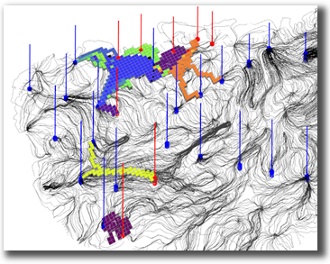
For a given time interval, studioSL will visualize the multipliers that will be applied to the chosen grid property. The locations of the multipliers are determined by the streamlines that support the wells at the specific time interval of mismatch, and the multiplier values reflect the extent of the mismatch at the selected wells for that particular time interval.
Automatic Running
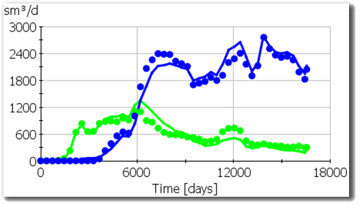
Once the wells, static properties, and time intervals are selected, studioSL will begin the history matching workflow. After each run up to time interval N, new corrections are computed and applied to the next run, which is restarted from time zero and progressed to time interval N+1. A summary plot of the history matching errors (objective function) or well-by-well rate mismatches can be generated to track the progress of the run.

Well and Properties Comparison


After processing all time intervals, it becomes straightforward to evaluate the history match improvements for all wells or to compare the grid properties before and after the history matching process.
Additional Features
- High resolution grids with 100's of wells and 100's of timesteps.
- Works with Eclipse .DATA models.
- Compare well vs field level matches among multiple runs.